Wold's decomposition theorem
The most fundamental justification for time series analysis (as described in this text) is due to Wold's decomposition theorem, where it is explicitly proved that any (stationary) time series can be decomposed into two different parts. The first (deterministic) part can be exactly described by a linear combination of its own past, the second part is a MA component of a finite order.
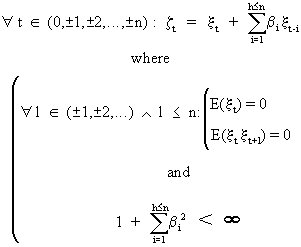
A slightly adapted version of Wold's decomposition theorem states that any real-valued stationary process Yt can be written as

(V.I.1-171)
where
yt
and zt
are not correlated.

(V.I.1-172)
where
yt
is deterministic

(V.I.1-173)
and

(V.I.1-174)
(zt
has an uncorrelated error with zero mean).
Because
of its importance for time series analysis in general, and in
practice, we will discuss the proof of Wold's decomp. theorem
shortly.
Since
there seems to be much confusion in literature about this theorem,
we will only discuss the proof of another version (than that
described above) which can be proved quite easily. In order to make
a distinction with the previous description, we will explicitly use
other symbols.
Denote
a stationary time series Wt with zero mean and finite
variance.
In
order to forecast the time series by means of a linear combination
of its own past

(V.I.1-175)
a
criterion is used to optimize the parameter values. This criterion
is

(V.I.1-176)
which
is called the sum of squared residuals (SSR).
The
normal equations (c.q. eq.
(V.I.1-176) differentiated w.r.t. the parameters) is easily found to
be

(V.I.1-177)
In
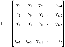
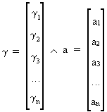
matrix notation eq. (V.I.1-177) becomes

(V.I.1-178)
with

(V.I.1-179)
which
is symmetric about both diagonals due to the stationary of Wt
and with

(V.I.1-180)
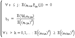
On
adding an error component et,n to eq.
(V.I.1-175) it can be shown that

(V.I.1-181)
The
first part of (V.I.1-181) is almost trivial

(V.I.1-182)
The
second part of (V.I.1-181) is

(V.I.1-183)
with
a RHS equal to zero since the parameters satisfy (V.I.1-177)
(Q.E.D.).
On
repeating the previous procedure we obtain

(V.I.1-184)
Remark
that the error components (V.I.1-181) and (V.I.1-184) are
uncorrelated due to (V.I.1-181), from which we obviously find

(V.I.1-185)
On
substituting (V.I.1-184) into (V.I.1-175) it is obvious that

(V.I.1-186)
where
xt,n(1)
depends on the past of Wt-1
Also
it is obvious from (V.I.1-183) that

(V.I.1-187)
and
from (II.II.1-27) and the fact that et,n
is independent from the other regressors of (V.I.1-186), that

(V.I.1-188)
On
repeating the step described above it is easy to obtain

(V.I.1-189)
with

(V.I.1-190)
On
applying (V.I.1-189) and (V.I.1-190) on Wt-i we obtain

(V.I.1-191)
where
xt-i,n
always depends on it's own past only, and where evidently

(V.I.1-192)
|

