m.
The behavior of non stationary time series
In
the previous subsections, non stationarity has been discussed at a
rather intuitive level. Now we will discuss some more fundamental
properties of the behavior of non stationary time series.
A
time series that is generated by

(V.I.1-213)
with
g(B)
an AR operator which is not stationary: g(B)
has d roots equal to 1; all other roots lie outside the unit circle.
Thus eq. (V.I.1-213) can be written by factoring out the unit roots

(V.I.1-214)
where
f(B)
is stationary.
In
general a univariate stochastic process as (V.I.1-214) is denoted an
ARIMA(p,d,q) model where p is the autoregressive order, d is the
number of non-seasonal differences, and q is the order of the moving
average components.
Quite
evidently, time series exhibiting non stationarity in both variance
and mean, are first to be transformed in order to induce a stable
variance, and then to be differenced enabling stationarity with
respect to the mean level. The reason for this is that power, and
logarithmic transformations are not always defined for negative
(real) numbers.
The
ARIMA(p,d,q) model can be expanded by introducing deterministic
d-order polynomial trends.
This
is simply achieved by adding a parameter - constant to (V.I.1-214),
expressed in terms of a (non-seasonal) non-stationary time series Zt
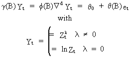
(V.I.1-215)

The
same properties can be achieved by writing (V.I.1-215) as an
invertible ARMA process

(V.I.1-216)
where
c is a parameter-constant. This is because
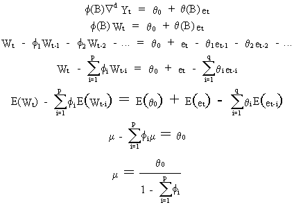
(V.I.1-217)

Also
remark that the p AR parameters must not add to unity, since this
would, according to (V.I.1-217), imply (in the limit) an infinite
mean level, an obvious nonsense!
An
ARIMA model can be generally written as a difference equation. For instance, the ARIMA(1,1,1) can be
formulated as

(V.I.1-218)
which
illustrates the postulated fact. This form of the ARIMA model is
used for recursive forecasting purposes.
The
ARIMA model can also be generally written as a random shock model
(c.q. a model in terms of the y-weights,
and the white noise error components) since

(V.I.1-219)
it
follows that

(V.I.1-220)
Hence,
if j is the maximum of (p + d - 1, q)

(V.I.1-221)
it
follows that the y-weights
satisfy

(V.I.1-222)
which
implies that large-lagged
y-weights
are composed of polynomials, exponentials (damped), and sinusoids
(damped) with respect to index j.
This
form of the ARIMA model (c.q. eq. (V.I.1-219)) is used to compute
the forecast confidence intervals.
A
third way of writing an ARIMA model is the truncated random shock
model form.

The
parameter k may be interpreted as the time origin of the observable
data. First, we observe that if Yt' is a particular
solution of
(V.I.1-213), thus if

(V.I.1-223)
then
it follows from (V.I.1-213), and
(V.I.1-223) that

(V.I.1-224)

Hence,
the general solution of (V.I.1-213)
is the sum of
Yt''
(c.q. a complementary function which is the solution of
(V.I.1-224)), and Yt' (c.q. a particular integral which
is a particular solution of
(V.I.1-213)).


(V.I.1-225)
and
that the general solution of the homogeneous difference equation with
respect to time origin k < t is
given by

(V.I.1-226)

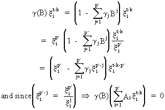
(V.I.1-227)


(V.I.1-228)
since
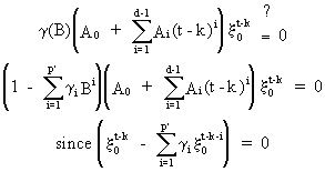
(V.I.1-229)
see
also (V.I.1-227).

The
general complementary function for

(V.I.1-230)
is

(V.I.1-231)
with
Di described in
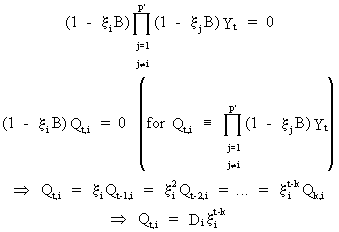
(V.I.1-232)
From
(V.I.1-231) it can be concluded that the complementary function
involves a mixture of:


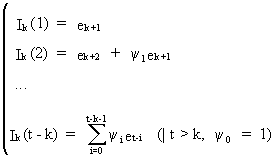
(V.I.1-233)
(with
y-weights
of the random shock model form) satisfying the ARIMA model structure
(where B operates on t, not on k)

(V.I.1-234)
which
can be easily proved on noting that

(V.I.1-235)
such
that

(V.I.1-236)

Hence,
if t - k > q eq. (V.I.1-233) is the particular integral of
(V.I.1-234).

If
in an extreme case k = -¥
then

(V.I.1-237)
called
the nontruncated random shock
form of the ARIMA model.


(V.I.1-238)
(compare
this result with (V.I.1-237)).
Also
remark that it is evident that

(V.I.1-239)


This
implies that when using the complementary function for forecasting
purposes, it is advisable to update the forecast as new observations
become available. | 
