II.II.1 OLS for Multiple Regression
The
general linear statistical
model can be described in matrix notation as

(II.II.1-1)
where
y is a stochastic T*1
vector, X is a
deterministic (exogenous) T*K matrix, b
is a K*1 vector of invariant parameters to be estimated by OLS, e
is a T*1 disturbance vector, T is the number of observations in the
sample, and K is the number of exogenous variables used in the right
hand side of the econometric equation.
It
is furthermore assumed
that

(II.II.1-2)
which
is the equivalent matrix expression of the weak set of assumptions
under section II.I.3.
The
least squares estimator minimizes e'e
(the sum of squared residuals).
Solving
the normal equations X'Xb
= X'y with respect to b
yields

(II.II.1-3)
where
X'X must be a non
singular symmetric K*K matrix!
Obviously,
the OLS estimator is unbiased

(II.II.1-4)
since
E(X'e) = 0
by assumption (X is
exogenous). This result can be proved quite easily.
Note that if X is not
exogenously given (thus stochastic) the small sample property of
unbiasedness only holds if E(X'e)
= 0.
Under
the assumption of OLS it can be proved that the covariance matrix of the parameters is

(II.II.1-5)
The
Gauss-Markov theorem
states that if
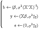
(II.II.1-6)
then
any other estimator

(II.II.1-7)
has
a parameter covariance matrix which is at least as large as the
covariance matrix of the OLS parameters

(II.II.1-8)
This
important theorem therefore proves that the OLS estimator is a best
linear unbiased estimator (BLUE).
If
D* is a K by T
matrix which is independent from y and if

(II.II.1-9)
the
parameter vector is by definition a linear estimator, and if

(II.II.1-10)
then
it follows that

(II.II.1-11)
Evidently,
it follows from (II.II.1-11) that the parameter vector can only be
unbiased if DX = 0
and if E(D*e) = 0.
Now
what happens to the covariance matrix of this estimator? Obviously,
we find
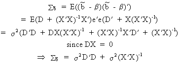
(II.II.1-12)
which proves the theorem (on comparing
(II.II.1-12) with (II.II.1-5); Q.E.D.).
It can be proved that

(II.II.1-13)
which
states that the OLS estimator of the variance is unbiased.
The
operational formula for calculating the variance
is

(II.II.1-14)
The
prediction of y
values outside the sample range is

(II.II.1-15)
which
is an unbiased
prediction function

(II.II.1-16)
Example of
extrapolation forecast
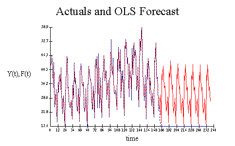
The
point forecast error can
be found as

(II.II.1-17)
whereas
the average forecast error
is equal to

(II.II.1-18)
The
degree of explanation can
be measured by the determination coefficient (R-squared) or by the
F-statistic which is defined as

(II.II.1-19)
and

(II.II.1-20)
and

(II.II.1-21)
where
the F statistic is valid
for all ß coefficients except for the constant term.
To
test the significance of a subset of m parameters (out of a total number of K) the following F
test is used

(II.II.1-22)
which
is in fact a generalization of (II.II.1-21).
The
parameter estimation of a multiple and a simple
regression are related to each other. It is also possible to
prove that if all explanatory variables are independent
(orthogonal), there is no difference between multiple and simple
regression coefficients. Assume
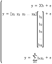
(II.II.1-23)

then
it is easily deduced from (II.II.1-23) that any multiple regression
parameter can be computed by
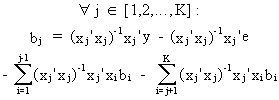
(II.II.1-24)
Since
it is assumed that the explanatory variables are orthogonal it
follows that

(II.II.1-25)
and
due to the OLS assumptions we know that

(II.II.1-26)
On
substituting (II.II.I-25) and (II.II.1-26) into (II.II.1-24) we
obtain

(II.II.1-27)
which
proves the theorem (Q.E.D.).
| 
