II.I.2 Ordinary Least Squares for Simple
Regression
Assume
the following relationship should be investigated by means of simple
linear regression
the
influence of the interest rate on the demand of new private
cars.
If
the researcher has two equally ranged time series, R for interest
rate) and C (for the demand of cars) the following mathematical
model could be considered:

(II.I.2-1)
This
is a linear relationship between C and R where ß is equal to the
sensitivity of C to R, alpha is equal to a constant term, and et
is equal to the error term.
Of
course one would expect beta to have a negative sign since high
interest rates would de-motivate potential car buyers, while low
interest rates would give them an incentive to buy more new cars
(due to cheaper loans).
It
is quite important to understand that in classic econometrics the
specification of the relationship to be considered such as eq.
(II.I.2-1) is based on economic theory (and common sense).
If
the necessary data (e.g. demand for new cars and interest rates) are
at hand, and if the researcher has a good economic specification,
all he needs is a mathematical technique to compute the
relationship.
Quite
often, econometrics is therefore defined as the intersection of
three sets: economic theory, economic statistics (data), and
mathematical techniques.
Before
we tackle the problem of computing a
and ß it must be understood that any technique of calculating the
parameters would generate some statistic error. This error will
occur because of the fact that the researcher only has two observed
time series which should be seen as a set of samples, drawn from a
population of all possible interest rates and all possible car sales
volumes (at any given moment in time). This is the reason why we
will never be able to calculate the true value of alpha and beta.
However, it is possible to estimate
the values of alpha and beta as good as possible (using the least
squares criterion).
We
rewrite the previous model by replacing alpha with the estimated
value of alpha and beta with the estimated value of beta:

(II.I.2-2)


Now
we will derive the formulae for the estimated alpha and beta for a
simple linear model (c.q. the estimator)

(II.I.2-3)
(assuming
a zero error component) and

(II.I.2-4)
Using
the first order condition it is possible to find a solution for both
parameters that minimize the SSR.
First
we calculate the partial derivative (of the SSR) with respect to
alpha and equate it to zero to find the optimum

(II.I.2-5)

(II.I.2-6)

(II.I.2-7)

(II.I.2-8)
where
in equation (II.I.2-7)

(II.I.2-9)
since

(II.I.2-10)
Secondly,
we calculate the partial derivative of the SSR with respect to beta
and equate it to zero

(II.I.2-11)

(II.I.2-12)

(II.I.2-13)

(II.I.2-14)
In practice eq. (II.I.2-8) and eq.
(II.I.2-14) are used to estimate the values of alpha and beta by the
so-called OLS technique. Remember that in case of parameter
estimation we replace the symbols alpha and beta by their estimated
values (these are indicated by a hat above the respective symbol).
In order to ensure that (II.I.2-5) and
(II.I.2-11)have been minimized (and not maximized) the second order
partial derivatives should be calculated. These derivatives will
have a positive sign (verify this). This proves that the two optima
we have found, do correspond with the minima of the SSR.
If a forecast of Yt has to be made, one
may use the following expression

(II.I.2-15)
where the estimated value of a from
(II.I.2-8) has to be replaced by

(II.I.2-16)
because we previously transformed the
exogenous variable according to eq. (II.I.2-4).
In this discussion of OLS we implicitly
made some crucial assumptions. If these assumptions are not
satisfied, OLS is not applicable.
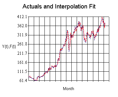
Example of an
interpolation forecast

| 
