|
When
two or more exogenous observation series are highly correlated or
have the same predictive power with respect to the endogenous variable they
are called multicollinear.


(III.IV-1)
which
means that both vectors are perfectly linearly
dependent (see eq. (I.IV-12)).
Multicollinearity
is a very serious problem, for instance if the researcher is
interested in calculating elasticities. If the only aim of the
researcher would be to generate forecasts, and if it would be
reasonable to assume that the multicollinearity problem would not be
different for the forecast period or cross-section, then
multicollinearity might be considered not to be a problem at all.
This is because multicollinearity will not affect the forecasts of a
model but only the weights of the explanatory variables in the
model.

It
is easy to show this mathematically. Assume a multiple regression
model with, among others, the two exogenous vectors from (III.IV-1)

(III.IV-2)
(see
eq. (II.II.1-1) and eq. (II.II.1-3)), then
it is obvious to see that X'X
must be a non singular
symmetric K*K matrix (see property (I.IV-14)).
Since
we assumed that

(III.IV-3)

For
this reason X'X is not
non-singular as well, and cannot be inverted (see properties of
section I.IV)! Therefore the b
vector of the OLS estimation cannot be computed. It should be noted
that other estimation methods like GLS, MLE, etc... will also fail.
So
far we 've discussed the effects of perfect multicollinearity. But what will happen when there is near
perfect multicollinearity?

(like
in eq. (I.IV-51)). The columns are
assumed to be the eigenvectors (corresponding to different latent
roots) of the square matrix A
(see eq. (I.IV-48)).
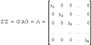
Since
GG' = I (see eq. (I.IV-47)) we can write
the linear model as

(III.IV-4)
where
the columns of Z are
called the principal components, which are orthogonal with respect to each
other and have a length equal to their eigenvalue.
Since
Z is symmetric and pos.
semi def., it follows that the eigenvalues are real (eq. (I.IV-37))
and nonnegative (see properties under section I.IV).
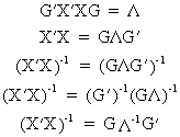
It
can easily be verified that

(III.IV-5)
which
follows from (I.IV-54), and agrees
with eq. (I.IV-30). Now we are
able to write the formula for the parameter vector

(III.IV-6)
and
more importantly, the parameter covariance matrix and variance

(III.IV-7)
from
which it can be deduced that if the eigenvalue corresponding to a
specific exogenous variable becomes small, the respective delta
coefficient will have a very large variance. In the extreme case
where the eigenvalue were to be zero, the variance would be
infinitely large (exact multicollinearity).
From
(III.IV-4) it follows

(III.IV-8)
and
from (III.IV-5)

(III.IV-9)
Now
the covariance matrix of the original b parameters can be written as

(III.IV-10)
which
not necessarily implies that low values for lambda yield high
variances (it also depends on the other parameters). Therefore, in
general, all is not lost when lambda is low (but it is possible).
| 
