IV.I.1
Formal derivation of demand systems
The
objective in non-probabilistic consumer behavior is to maximize
utility such that a budget constraint is satisfied. If U(q)
is twice continuously differentiable (then the Hessian of U(q) is symmetric and) then it is possible to obtain a Marshallian
demand function q = q(m,
p) (which is dependent on the known budget m and a known price
vector p (h*1)) where q
(h*1) contains the consumption quantities for a set of h commodities
such that U(q) reaches a maximum subject to p'q = m:

(IV.I.1-1)
The
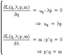
optimization problem can be formulated as a Lagrange function

(IV.I.1-2)
The
first order conditions are

(IV.I.1-3)
Remark
that it is implicitly assumed that U(q)
is stationary in its optimum and that all marginal utilities are
positive.
Since
the marginal utilities and (obviously also) prices are strictly
positive, the Lagrange multiplier (in (IV.I.1-3)) must be positive
as well.
The
second order condition must be satisfied in the maximum:

(IV.I.1-4)
It
can be shown that under strict quasi-concavity of utility (c.q.
strict convexity of the iso-utility curves), that (IV.I.1-4) is
satisfied.
It
can also be shown that a unique solution exists for q
= q(m, p), and the Lagrange multiplier, for which the solution follows from
(IV.I.1-3) as

(IV.I.1-5)
where
q* = q(m, p).
Obviously
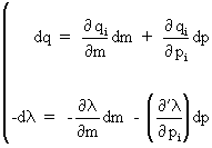
(IV.I.1-3) can be written as a differential

(IV.I.1-6)
or

(IV.I.1-7)
where
H* is the
Hessian matrix of the utility function U(q*).
On
noting that we already defined

(IV.I.1-8)
and
if we define

(IV.I.1-9)
it
is possible to write

(IV.I.1-10)
or
equivalently

(IV.I.1-11)
We
interpret qm as the vector of marginal income
sensitivities of consumption, and Qp as the matrix of
marginal price sensitivities of consumption. Remark that the
diagonal elements of Qp are the price sensitivities,
whereas the off-diagonal elements are the cross-price
sensitivities.
By
combining (IV.I.1-7) and (IV.I.1-11) we find

(IV.I.1-12)
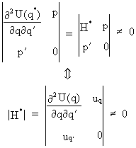
It
is possible to prove that q
= q(m, p) is continuously differentiable if and only if

(IV.I.1-13)
so
that the property of differentiability holds if the Hessian of the
utility function is non-singular.
It
can be shown that if U(q)
is assumed to have a decreasing marginal rate of substitution (MRS)
that H* is non-singular. Therefore if U(q) has a diminishing MRS, the demand equations are continuously
differentiable.
Since
we know that H*
is a symmetric matrix, it follows that

(IV.I.1-14)
is
also symmetric.
On
substituting (IV.I.1-14) into (IV.I.1-12) we find

(IV.I.1-15)
In
(IV.I.1-15) it is quite obvious to see that

(IV.I.1-16)
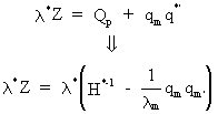
Furthermore
we can rewrite (IV.I.1-14) as

(IV.I.1-17)
thus

(IV.I.1-18)
and

(IV.I.1-19)
and

(IV.I.1-20)
and

(IV.I.1-21)
Now
it follows from (IV.I.1-18) and (IV.I.1-19) that

(IV.I.1-22)
which
implies that Z is symmetric (since H*
is symmetric). Above this the inverse of the Hessian matrix has negative
diagonal elements which is equivalent to saying that the
indifference curves are convex (see (IV.I.1-4)).
Equation
(IV.I.1-20) implies homogeneity
meaning that substitution effects are in fact a reallocation of
goods without changing the overall level of consumption. Therefore
only the relative price changes are important for substitution
effects.
In
(IV.I.1-21) the adding up property is illustrated. All prices multiplied by their
respective propensity to consume sum up to one (i.e. a weighted sum
of budget elasticities of demand).
From
(IV.I.1-11) we find quite easily

(IV.I.1-23)
Partial
substitution of (IV.I.1-15) into
(IV.I.1-23) yields

(IV.I.1-24)
From
(IV.I.1-16) equation (IV.I.1-24)
becomes

(IV.I.1-25)
Substituting
(IV.I.1-22) into (IV.I.1-25) gives

(IV.I.1-26)
which
is the structural form of our (general) demand system where the
first term is attributed to the income
effect whereas the second term takes the substitution
effect into account.
The
substitution effect, due to Hicks and Allan, is given by
 . .
This
can be shown quite easily by using (IV.I.1-15) and (IV.I.1-16)

(IV.I.1-27)
which
is just a "compensated price effect" (due to Hicks). In
micro economics the Hicksian demand function is equal to the
Marshallian function which is "compensated" for the change
in real income (such that the original utility level is attained).
Thus
from (IV.I.1-27) and (IV.I.1-22) we obtain

(IV.I.1-28)
and
thus the second term of (IV.I.1-26) represents the substitution
effect. | 
