V.I.5
Some remarks and model extensions of the ARIMA model
a.
Seasonality
The
previously described techniques (for ARIMA model building) can be
easily expanded for seasonal time series. In fact all
identification, estimation, checking, and forecasting procedures are
not different from the non-seasonal counterpart. All the above
descriptions and reflections are still valid for the seasonal case:
one only has to substitute the time lag i (in t-i) for i*s (to
obtain an index t-i*s) where s is the seasonal period (e.g. s = 12
for monthly, and s = 4 for quarterly data).
There
are two possible ways to combine the non-seasonal and seasonal ARIMA
structures into one model.
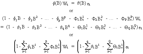
First
an additive seasonality model could be considered

(V.I.5-1)


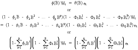
Second,
a multiplicative seasonality model could be considered

(V.I.5-2)
which
is a model containing several (implicit) restrictions on the
parameters. This is the standard model which is used, because it
takes into account the interaction between seasonal and non-seasonal
ARIMA structures: this can be seen by the simple fact that seasonal
and non-seasonal parameters are multiplied (on writing the explicit
forecast function).

b.
Nonlinearity
ARIMA
models are capable of modeling some nonlinearities, since they
involve (if a seasonal or non-seasonal MA part is present) rational
lag structures in terms of the error

(V.I.5-3)
Due
to Wold's decomp. theorem this should suffice to model a
stationary time series adequately. It is however possible that
another (nonlinear) specification yields a better model, w.r.t.
parameter parsimony for certain time series (e.g. a combination of
some distributed lag models).
The
main reason however, why these alternatives are not successful, is
the simple fact that ARIMA models can be built according to the
Box-Jenkins methodology which is a comprehensive, general, and
widely applicable procedure, involving many possible diagnostic
identification tools; theoretical (mathematical) structures that are
easily proved; many checking procedures; and means for model
criticism, monitoring, and control. Above that, the Box-Jenkins
methodology also suggests means of expanding ARIMA models with the
information of exogenous variables (c.q. transfer function).
c.
Variable parameters and the Kalman Filter
It
is possible to model and estimate ARIMA models where the ARMA
parameters (and sometimes even the l parameter) are simultaneously
estimated, allowing for (smooth) parameter changes over time. This
can be done on using a recursive approach (c.q. estimating
parameters for a short sample, and iteratively expanding by one
observation such that the parameters can be re-estimated), or on
using the famous recursion formulae due to Kalman (see also HARVEY
1989, and his program STAMP). | 
