V.I.4
Univariate Stochastic ARIMA Model Forecasting
The
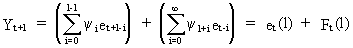
forecast (with forecast lead l) of a time series Yt at a
forecast origin t is denoted by Ft+l or Ft(l)
which is, in our case, always a combination of previous
observations.
The
forecast can obviously also be written in terms of previous
error-shocks
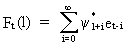
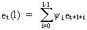
(V.I.4-1)

Remark
that from (I.III-17) it follows
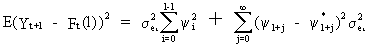
that the forecast variance is

(V.I.4-2)

and
due to (V.I.1-238) and (V.I.1-233)
it follows that
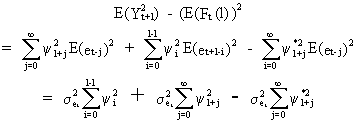
(V.I.4-3)

(V.I.4-4)

(V.I.4-5)
Hence,
the forecast function (c.q. the conditional expectation of Yt+l
at t) is the minimum mean square error forecast. Also it is
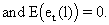
quite evident that the forecasts are unbiased
since
(V.I.4-6)
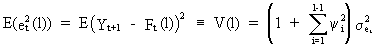
The
variance of the forecast is equal to the first term of the RHS of
(V.I.4-4). This illustrates why (V.I.1-51)
(and especially the y-weights)
can be used to compute the forecast confidence interval.
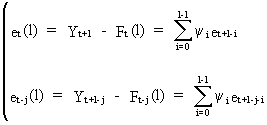
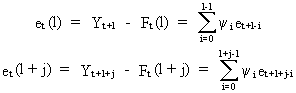
It
is furthermore nice to see that the random innovations (c.q. shocks)
are in fact equivalent to the one
period ahead forecast error since

(V.I.4-7)
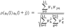
From
(V.I.4-5) and (V.I.4-7) it follows that the one step ahead forecast
errors are not correlated. Remark however that forecast errors for l
> 1 are not uncorrelated.
There
are two formulae for computing the correlations
between forecast errors (l > 1): correlations between
forecast errors at different origins with equal lead times, and
correlations between forecast errors at equal origins with different
lead times.
(Auto)correlations
between forecast errors at different origins with equal leads
are given by
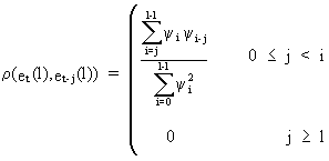
(V.I.4-8)
which
can be easily proved on using
(V.I.4-9)


(V.I.4-10)
which
proves (V.I.4-8) (Q.E.D.).
(Auto)correlations
between forecast errors at equal origins but with different
leads are given by
(V.I.4-11)
since
(V.I.4-12)
Hence,
the covariance is
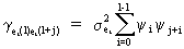
(V.I.4-13)
which,
together with (V.I.4-12), proves (V.I.4-11) (Q.E.D.).
Forecasting
of ARIMA(p,d,q) models

(V.I.4-14)
is
straightforward since
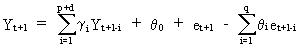
(V.I.4-15)
from
which it follows that
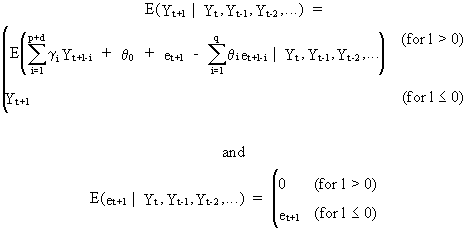
(V.I.4-16)
Eq.
(V.I.4-15) provides a recursive
forecasting algorithm which can be solved using a computer and a
programming language able to perform recursions.
The
forecast variances (and
hence also the confidence probability limits) can be obtained from
the y-weights.
These
y-weights
are computed from
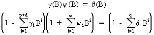
(V.I.4-17)
which
can be used to equate coefficients of powers of B such that
(V.I.4-18)

Remark
that if j > max(p + d - 1, q) eq. (V.I.4-18) reduces to
(V.I.4-19)
Sine
the variance of the forecast is equal to the first term of the RHS
of (V.I.4-4), it follows that
(V.I.4-20)
Confidence
intervals can thus also be easily obtained.
Some
explicit examples of the so-called eventual
forecast functions are given in BOX and JENKINS (1976) and in
MILLS (1990). These functions are used to study the fundamental
nature of the forecasts. Since this goes beyond the scope of this
work, and since the fundamental techniques of studying these
forecast functions has already been given in previous sections, we
only refer to the relevant literature. |